3.1.1. crysolの実行
crysolのヘルプを表示させてみると、
[ ]:
!crysol -h
[ ]:
  Usage in the batch mode:
  crysol [<Inp_File1>]...[<Inp_FileK>] [<Dat_File>]
  [-param1 <param1>]...[-paramN <paramN>]

    :
  途中略
    :

  Examples:

  crysol 6lyz.pdb -lm 20
  Calculate scattering intensity from the PDB file
  6lyz.pdb with Lmax = 20 and without fitting

  crysol mod*.pdb exp.dat -un 2
  Process PDB files with the names beginning with
  "mod" and fit experimental data exp.dat with
  scattering vector given in inverse nanometres.

  crysol *.sav lyzexp.dat
  Restore the scattering intensity from all
  sav files in the current directory and fit
  the experimental data in the file lyzexp.dat

Report bugs to <atsas@embl-hamburg.de>.
ご覧のように、コマンド実行の結果がセルとして表示されているのがわかる。
今、リゾチウムの結晶構造から 6lyz.pdb を計算してみよう。 crysol の引数はデータ点数を201とするために -ns 201 としている。
[ ]:
!crysol 6lyz.pdb -lm 20 -ns 201
[ ]:
***  ------------------------------------------------  ***
  ***    C R Y S O L  Wintel/UNIX/Linux version 2.8.4    ***
  ***  Please reference: D.Svergun, C.Barberato          ***
  ***   & M.H.J.Koch (1995) J. Appl.Cryst., 28, 768-773  ***
  ***   Version (LMAX=99) for small and wide angles      ***
  ***        Last revised  ---  10/12/18 10:00           ***
  ***   Copyright (c) ATSAS Team                         ***
  ***   EMBL, Hamburg Outstation, 1995 - 2018            ***
  ***  ------------------------------------------------  ***

  ------------------------------------------------
                  Program options :
  0 - evaluate scattering amplitudes and envelope
  1 - evaluate only envelope and Flms
  2 - read CRYSOL information from a .sav file
   Type crysol -help for batch mode use
  ------------------------------------------------

  ------------------------------------------------
          Following file names will be used:
 6lyz01.log -- CRYSOL log-file          (ASCII)
 6lyz01.int -- scattering intensities   (ASCII)
 6lyz01.alm -- net partial amplitudes   (binary)
  ------------------------------------------------
  ----------  Reciprocal space grid  -------------
   ( in s = 4*pi*sin(theta)/lambda [1/angstrom] )
 Read atoms and evaluate geometrical center ...
  Number of atoms read .................................. : 1001
  Number of discarded waters ............................ : 101
 Percent processed      10  20  30  40  50  60  70  80  90 100
 Processing atoms   :>>>>>>>>>>>>>>>>>>>>>>>>>>>>>>>>>>>>>>>>
 Center of the excess electron density:  0.452 -0.004  0.276
 Processing envelope:>>>>>>>>>>>>>>>>>>>>>>>>>>>>>>>>>>>>>>>>
 Processing envelope:>>>>>>>>>>>>>>>>>>>>>>>>>>>>>>>>>>>>>>>>
 --- Structural parameters (sizes in angstroms) ---
 Electron   rg   :  13.99       Envelope   Rg      :  14.08
 Shape      Rg   :  13.97       Envelope  volume   : 0.1806E+05
 Shell    volume : 0.1129E+05   Envelope  surface  :  3150.
 Shell      Rg   :  18.98       Envelope  radius   :  25.49
 Shell    width  :  3.000       Envelope  diameter :  49.04
 Molecular weight: 0.1432E+05   Dry volume         : 0.1736E+05
 Displaced volume: 0.1741E+05   Average atomic rad.:  1.607
 Number of residuals :   129
 Average atomic volume .................................. : 17.40
 Rg ( Atoms - Excluded volume + Shell ) ................. : 15.04
 Rg from the slope of net intensity ..................... : 15.41
 Average electron density ............................... : 0.4383
 Intensities    saved to file 6lyz01.int
 I_abs(s)[cm^-1]/c[mg/ml] saved to file 6lyz01.abs
 Net amplitudes saved to file 6lyz01.alm
abs 、 alm 、 int それにプログラムのログである log という拡張子のファイルが crysol 実行毎に生成される。
散乱曲線のデータは abs と int であるが使うのは int の方である。
実際にファイルの中身を一部表示させると、
[ ]:
!head "6lyz00.int"
[ ]:
 Dif/Atom/Shape/Bord 6lyz.pdb     Dro:  0.030 Ra: 1.6074 Rg: 15.41 Vtot:  18057.
  0.000000E+00  0.484317E+07  0.582674E+08  0.338289E+08  0.147208E+06
  0.250000E-02  0.484078E+07  0.582433E+08  0.338151E+08  0.147088E+06
  0.500000E-02  0.483365E+07  0.581719E+08  0.337741E+08  0.146731E+06
  0.750000E-02  0.482179E+07  0.580530E+08  0.337059E+08  0.146137E+06
  0.100000E-01  0.480523E+07  0.578869E+08  0.336106E+08  0.145308E+06
  0.125000E-01  0.478402E+07  0.576741E+08  0.334884E+08  0.144250E+06
  0.150000E-01  0.475822E+07  0.574149E+08  0.333397E+08  0.142965E+06
  0.175000E-01  0.472792E+07  0.571101E+08  0.331648E+08  0.141462E+06
  0.200000E-01  0.469315E+07  0.567603E+08  0.329640E+08  0.139740E+06
ここで最初の行は理論散乱曲線を計算するためのパラメータで、使用するのは 1列目の \(q\) と2列目の \(I(q)\) のみである。残念ながらcrysolの出力はすぐ使えるようになっていないので加工して保存してやる必要がある。
3.1.2. 理論データの保存
さっそくこのファイルを読み込んでみよう。普通にpythonでファイルを読むこともできるが、せっかくなので、 pandas (https://pandas.pydata.org/) と呼ばれるpythonで データ解析を行うためのパッケージを使ってみる。
pandasには1次元のSeriesと2次元のDataFrameという2つのデータ構造が用意されているが、小角では普通DataFrameを使う。
pandasだけでなく描画や数値計算など必要なモジュールをインポートしておく
[1]:
%matplotlib inline
import numpy as np
import pandas as pd
import matplotlib.pyplot as plt
タンパク質溶液散乱の場合、散乱強度 \(I(q)\) は重量濃度 \(c\) で割った形で実験値として使用するので、2列目の \(I(q)\) を分子体積 Vtot で割っておく。
Vtot は header に書きこまれているので、最初に Vtot だけ取り出しておく。
[2]:
f=open("6lyz00.int")
header=f.readline()
Vtot=float(header.split(":")[-1])
print('Vtot=',Vtot)
Vtot= 18057.0
[3]:
df=pd.read_csv("6lyz00.int",delim_whitespace=True,header=0,names=["q","I"],usecols=[0,1])
[4]:
df
[4]:
| q | I | |
|---|---|---|
| 0 | 0.0000 | 4843170.0 |
| 1 | 0.0025 | 4840780.0 |
| 2 | 0.0050 | 4833650.0 |
| 3 | 0.0075 | 4821790.0 |
| 4 | 0.0100 | 4805230.0 |
| ... | ... | ... |
| 196 | 0.4900 | 24998.3 |
| 197 | 0.4925 | 24965.8 |
| 198 | 0.4950 | 24943.6 |
| 199 | 0.4975 | 24931.3 |
| 200 | 0.5000 | 24928.1 |
201 rows × 2 columns
先程書いたように \(I(q)\) を \(I(q)/c\) に対応させるために2列めに\(I(q)/Vtot\)、3列目には各点の誤差を入れるのが小角散乱における標準フォーマット なので仮想的に\(I(q)\)の3%の値を入れておく。
[5]:
df["I"]=df["I"]/Vtot
df["sI"]=df["I"]*3./100
df
[5]:
| q | I | sI | |
|---|---|---|---|
| 0 | 0.0000 | 268.215650 | 8.046470 |
| 1 | 0.0025 | 268.083292 | 8.042499 |
| 2 | 0.0050 | 267.688431 | 8.030653 |
| 3 | 0.0075 | 267.031622 | 8.010949 |
| 4 | 0.0100 | 266.114526 | 7.983436 |
| ... | ... | ... | ... |
| 196 | 0.4900 | 1.384410 | 0.041532 |
| 197 | 0.4925 | 1.382611 | 0.041478 |
| 198 | 0.4950 | 1.381381 | 0.041441 |
| 199 | 0.4975 | 1.380700 | 0.041421 |
| 200 | 0.5000 | 1.380523 | 0.041416 |
201 rows × 3 columns
このようにして作ったdfをファイル6lyz.datに出力する。 header行だけ先に書いておき
[6]:
f=open("6lyz.dat","w")
headerline="# q     I(q)     sI(q)\n"
f.write(headerline)
f.close()
次にdataを追記する。フォーマットは指定できる。
[7]:
df.to_csv("6lyz.dat",sep=' ',mode="a",float_format='%.6e', header=False, index=False)
ファイルの中身は
[ ]:
!head "6lyz.dat"
[ ]:
# q     I(q)     sI(q)
0.000000e+00 2.682157e+02 8.046470e+00
2.500000e-03 2.680833e+02 8.042499e+00
5.000000e-03 2.676884e+02 8.030653e+00
7.500000e-03 2.670316e+02 8.010949e+00
1.000000e-02 2.661145e+02 7.983436e+00
1.250000e-02 2.649399e+02 7.948197e+00
1.500000e-02 2.635111e+02 7.905333e+00
1.750000e-02 2.618331e+02 7.854993e+00
2.000000e-02 2.599075e+02 7.797225e+00
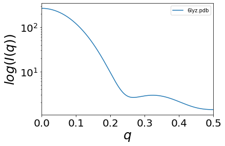
3.1.3. データのプロット
データのプロットはpythonのmatplotlib (https://matplotlib.org/) を使うのが一般的である。 縦軸に\(I(q)\)の対数を取る。
[9]:
ax=df.plot(x='q',y='I',logy=True,fontsize=20,label='6lyz.pdb')
ax.set_xlabel('$q$',fontsize=25)
ax.set_ylabel('$log(I(q))$',fontsize=25)
#plt.savefig('Iq.png')
[ ]: